Tensor Parallelism

Introduction

Tensor parallelism is a form of Model Parallelism. It makes it possible to use models that would be to large for a single GPU’s VRAM by sharding the model between multiple GPUs. It can also speed up training and inference by performing work in parallel on multiple GPUs.

Splitting matrices

Tensor parallelism works by dividing up weight matrices into blocks by splitting them on rows or columns. Each GPU then performs matrix multiplication using its own block of the weight matrix. After matrix multiplication, the results from each GPU can be joined again.

We can split the operands to matrix multiplications in several ways. These different splitting ‘patterns’ will turn out to be useful for different neural network layers, so later sections will revisit them. The different splitting patterns follow naturally from the definition of matrix multiplication.

For a matrix multiplication $C=AB$, the cell $C_{i,j}$ is calculated as $C_{i,j}=A_{i,\ast }\cdot B_{\ast ,j}={\sum }_{h=1}^k{A}_{i,h}{B}_{h,j}$. So, a cell $C_{i,j}$ is the result of the dot product of the $i$-th row of $A$ and the $j$-th column of $B$. For example, to calculate $C_{2,1}$ in the example below, we calculate the dot product of $A_{2,\ast }$ and $B_{\ast ,1}$ (cell and vectors are in a darker shade):

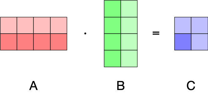
Since the dot products are between rows of $\mathbf{A}$ and columns $\mathbf{B}$, we can split the rows of $\mathbf{A}$ between GPUs and we will still get correct results:

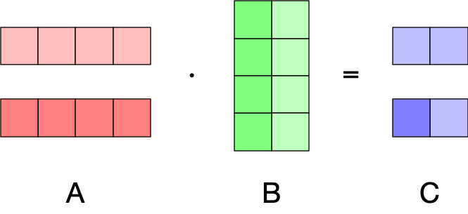
The only catch each GPU will only have a subset of the rows of $\mathbf{C}$. We can obtain the matrix $C$, by concatenating the results from each GPU.

Similarly, we could split the columns of matrix $B$:

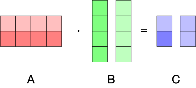
Can we split both the rows of $A$ and the columns of $B$? Try it out!

Another pattern that will prove very useful is that we could split the columns of $A$ and rows of $B$:

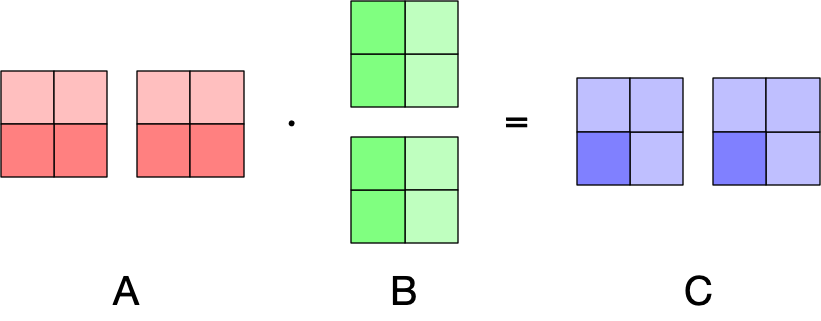
This works as long as we put the $n$-th column split of $A$ on the same GPU as the $n$-th row split of $B$. This will result in two output matrices, both with the same shape as $C$. However in this case, the first GPU will have the partial dot product $A_{i,1}{B}_{1,j}+A_{i,2}{B}_{2,j}$ for cell $C_{i,j}$ and the second GPU the partial dot product $A_{i,3}{B}_{3,j}+A_{i,4}{B}_{4,j}$. Since the dot product operation sums over pairwise vector component multiplications, we can obtain the result of $C_{i,j}$ by summing the partial dot products. In other words, we can calculate $C$ by summing the GPU output matrices element-wise.

This turns out to be a very powerful pattern, particularly if we have two linear layers that are subsequently applied at described in the Tensor parallelism in transformers section.

Here is a short piece of code using Torch that simulates this splitting pattern with slightly larger matrices:^[Done on one device for simplicity.]

import torch
 
# Non-split matrices used for verification.
A = torch.rand(16, 32)
B = torch.rand(32, 8)
C = A @ B
 
# Split A along columns, B along rows, then:
#
# GPU 1: A1, B1
# GPU 2: A2, B2
A1, A2 = A.chunk(2, dim=1)
B1, B2 = B.chunk(2, dim=0)
C1 = A1 @ B1
C2 = A2 @ B2
 
# Verify that the result is the same after an element-wise sum.
torch.testing.assert_close(C, C1 + C2)

Tensor parallelism in transformers

Feed-forward layers

For a given feature vector $x$, a transformer’s feed-forward layer applies the transformation: $h=g(xW)V$ where $W$ projects $x$ to a higher dimensionality, $g$ is a non-linear activation function, and $V$ is a matrix that projects $g(xW)$ to a lower dimensionality. Since we apply a transformer to multiple sequences and multiple tokens within a sequence, we use $X$ with shape [batch_size * seq_len, hidden_size] instead.

To applying tensor parallelism, we start with the innermost expression $XW$. There are two restrictions that we have to work with:

1. $X$ is usually not split across GPUs, so each GPU will have the full input matrix.
2. For non-linear activation functions, there is no function $f$, such that $g(a+b)=f(g(a),g(b))$. In other words, when splitting $W$ for tensor parallelism into $W^1$ and $W^2$, we have to ensure that $X{W}^{(1)}$ and $X{W}^{(2)}$ contain full dot products that $g$ can be applied to.

Given these restrictions, we want to split $W$ along the columns (see Splitting matrices), so we can use the following pattern from Splitting matrices (where $X=A$ and $W=B$):

Since the resulting split matrices contain full dot products, we can apply the activation function $g$ without issues. Next, we want to matrix-multiply $g(xW)$ with $V$. To do so, we can split $V$ along its rows, using the following pattern (where $g(xW)=A$ and $V=B$):

Then we can sum the resulting matrices from the two GPUs element-wise to obtain the final result.

Tensor parallelism with PyTorch Linear The PyTorch Linear layer uses a matrix with shape [out_features, in_features] internally. So if you are writing a weight loader that supports tensor parallelism in PyTorch, you have to update the splitting accordingly.

Feed-forward layers with gating

Some newer transformers architectures use a gating mechanism in the feed-forward layer:

$h=(g(xW)\cdot xU)V$ This doesn’t fundamentally change the approach to tensor parallelism — $xW$ is split as before and when $xU$ is split in the same manner, the element-wise multiplication can be performed on the same GPU.

Attention layers

Recap

To understand tensor parallelism in Scaled Dot-Product Attention, we briefly revisit the SDPA equations and shapes. The simplified formulation of SDPA is:

$\text{Attention}(Q,K,V)=\text{softmax}(\frac{Q{K}^T}{\sqrt{d_k}})V$ Here, $Q$, $K$, and $V$ are the query key and value representation of the inputs (more about that in a bit) and $d_k$ is the dimensionality of the query and key representations. In this simplified equation, the shape of $Q,K,V$ is [batch_size, seq_len, hidden_size]. Finally, the result of attention is transformed using an output matrix $W^O$:

$\text{Attention-Layer(Q,K,V)}=\text{Attention}(Q,K,V)W^O$

The actual transformer architecture uses multi-head self attention. That is, the transformers has $h$ attention heads^[Some later extensions of the transformer use a different number of key/value heads than query heads.] and there are different query, key, and value representations of the head:

$\text{MultiAttention}(Q,K,V)=\text{Concat}({\text{head}}_1,\dots ,{\text{head}}_h)$ $\text{where}{\text{head}}_i=\text{Attention}(Q_i,K_i,V_i)$

where $Q_i,K_i,V_i$ have shape [batch_size, seq_len, head_size] where typically n_heads*head_size==hidden_size. The head-specific query, key, and value are calculated from the input $X$:

$Q_i=X{W}_i^Q,K_i=X{W}_i^K,V_i=X{W}_i^V$

Where each weight matrix has shape [hidden_size, head_size]. Since every head is computed independently, it provides a great opportunity for parallelization.

Optimization

Since doing separate matrix multiplications per-head is not very efficient, most transformer implementations will process all the heads at the same time by concatenating the heads representations. So, the head representations of $Q,K,V$ are calculated at the same time:

$Q=X{W}^Q,K=X{W}^K,V=X{W}^V$ The shape of each weight matrix is [hidden_size, n_heads * head_size]. So, throughout SDPA the shapes are as follows:

• $Q,K,V$ have the shape [batch_size, seq_len, n_heads * head_size].
• $Q,K,V$ are permuted to [batch_size, n_heads/n_splits, seq_len, head_size]. This is done so that the following operations are by head.
• $Q{K}^T$ in $\text{MultiAttention}$ results in the shape [batch_size, n_heads, seq_len, seq_len], these are the unnormalized attention matrices.
• $\text{softmax}(\frac{Q{K}^T}{\sqrt{d_k}})$ normalization does not change the shape.
• $\text{softmax}(\frac{Q{K}^T}{\sqrt{d_k}})V$ results in the shape [batch_size, n_heads, seq_len, head_size]
• The the shape is permuted to [batch_size, seq_len, (n_heads * head_size)] to get $\text{MultiAttention}(Q,K,V)$).
• To get the output of the layer, we calculate $\text{MultiAttention}(Q,K,V)W^O$. Since $W^O$ has the shape [n_heads*head_size, hidden_size], the output of the attention layer has the shape [batch_size, seq_len, hidden_size].

Tensor parallelism

As mentioned before, since the heads are computed separately, we can compute them in parallel. For instance, when a model has 16 heads and we have 2 GPUs, we could perform multi-head attention for 8 heads on each GPU.

Since the columns of $W^Q$, $W^K$, and $W^V$ are ordered by heads, we can split each on the columns for tensor parallelism, as long as the partitioning does not split any heads. So, calculating $Q,K,V$ has the following pattern (modulo batching),

where $X=A$, $W^Q,W^K,W^V=B$, and $Q,K,V=C$

The following then happens in terms of shapes (where tp is the number of GPUs):

• $Q,K,V$ have the shape [batch_size, seq_len, (n_heads * head_size)/tp].
• $Q,K,V$ are permuted to [batch_size, n_heads/tp, seq_len, head_size].
• $Q{K}^T$ results in the shape [batch_size, n_heads/tp, seq_len, seq_len].
• $\text{softmax}(\frac{Q{K}^T}{\sqrt{d_k}})$ normalization does not change the shape.
• $\text{softmax}(\frac{Q{K}^T}{\sqrt{d_k}})V$ results in the shape [batch_size, n_heads/tp, seq_len, head_size]
• The the shape is permuted to [batch_size, seq_len, (n_heads * head_size)] to get $\text{MultiAttention}(Q,K,V)$).

Now we can compute the final output of the attention layer as $\text{Attention-Layer(Q,K,V)}=\text{Attention}(Q,K,V)W^O$. Since $\text{Attention}(Q,K,V)$ is split by column, we can split $W^O$ by its rows to use the following pattern:

where $A=\text{MultiAttention}(Q,K,V)$, $B=W^O$ and $C$ is the layer output. Then we can sum $C$ from the each GPU element-wise to obtain the final result.

Other Q:KV head mappings

So far, this section has talked about multi-head attention in which there is an equal number of query, key, and value heads. However, there are other possible mappings, see Head mapping variants for a more extensive discussion.

This section covers the ramifications of these variants briefly for tensor parallelism.

Multi-Query Attention is the easiest case, the query and thus the query weight matrix $W^Q$ can be split as above. Since the single key/value heads need to interact with all the query heads, $K$ and $V$ and thus the weights $W^K$ and $W^V$ need to be placed fully on all GPUs.

For Multi-Query Attention we need to ensure that the key/value heads are on the same GPU as the query heads that they are mapped to. This turns out to be easy as long as the number of key/value heads can be divided evenly by the amount of parallelism (GPUs) and the amount of parallelism is not larger than the number of key/value heads. In this case we can split $W^Q$, $W^K$, and $W^V$ evenly in the same number of chunks. For instance, if we split the example in the image above across 2 GPUs, we can split the query heads evenly in 4 heads per GPU and the key/value heads evenly in 2 heads per GPU, and the mapping will still be correct.